
You are here
Science blog of a physics theorist Feed

The Standard Model More Deeply: The Electron and its Cousins (Part 1)
[This is a follow-up to Monday’s post, going more into depth.]
Among the known elementary particles are three cousins: the electron, the muon and the tau. The three are identical in all known experiments — they have all the same electromagnetic and weak nuclear interactions, and no strong nuclear interactions — except that they have different rest masses:
- electron rest mass: 0.000511 GeV/c2
- muon rest mass: 0.105658 GeV/c2
- tau rest mass: 1.777 GeV/c2
[These differences arise from their different interactions with the Higgs field; to learn more about this, see Chapter 22 of my book.]
Question: How sure are we that these three cousins aren’t actually the same object, seen in three different quantum states?
Quantum StatesThis is a serious possibility, at first glance. After all, individual atoms have many states, in which they look roughly the same but have different energies — which means, because E=mc2, that they have different rest masses. In Fig. 1 are some of a hydrogen atom’s many possible states; the one of lowest energy is called the “ground state”, and ones with more energy are referred to as “excited states”.
Figure 1: Energy levels of quantum states of a hydrogen atom. The lowest-energy state, at far left, is the ground state; all others are excited states. (The energy, measured in electron-volts and negative, is expressed relative to the amount of energy stored in a proton and an electron when the two are fully separated.) Might the electron, muon and tau similarly be three states of the same object?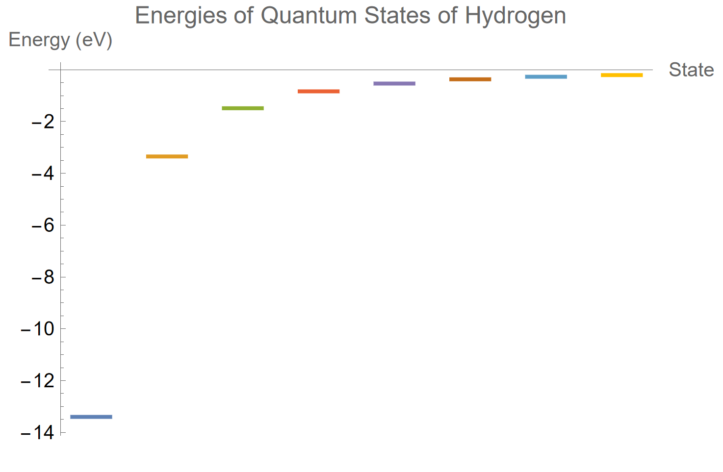
In a number of ways, hydrogen atoms in these different states are almost the same; each has zero electric charge, and each contains an electron and a proton. They differ in what the electron is doing, as sketched in Figure 2.
Figure 2: How the electron in hydrogen spreads out in different states. Upper left is the ground state; the other five are examples of excited states. Image from https://en.wikipedia.org/wiki/File:HAtomOrbitals.png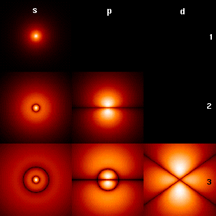
From the outside, though, they seem almost the same; the most obvious difference is that they have different amounts of energy. Might the electron, similarly, be the ground state of a complex object, with the muon and tau being that object’s most easily accessible excited states?
I’ve already mentioned one of the facts in favor of this hypothesis: the three particles’ identical interactions with all fields (except the Higgs field). Another hint that might support the hypothesis is this: when a muon or tau “decays” (i.e. when it transitions, via dissipation, to more stable particles), the outcome always includes an electron. For instance, the muon decays to an electron, a neutrino and an anti-neutrino. Tau decays are more complex, but in the end, an electron is always found among its decay products.
Nevertheless, the hypothesis is definitely wrong, as we can see by carefully comparing atoms, electrons, and protons. I’ll do this in two stages:
- Today I’ll describe what we learn from collisions of these particles.
- Soon I’ll describe what we learn from “spin” — angular momentum carried by a particle.
Let’s look at two typical ways to excite an atom; there are many others, but these two will do for today.
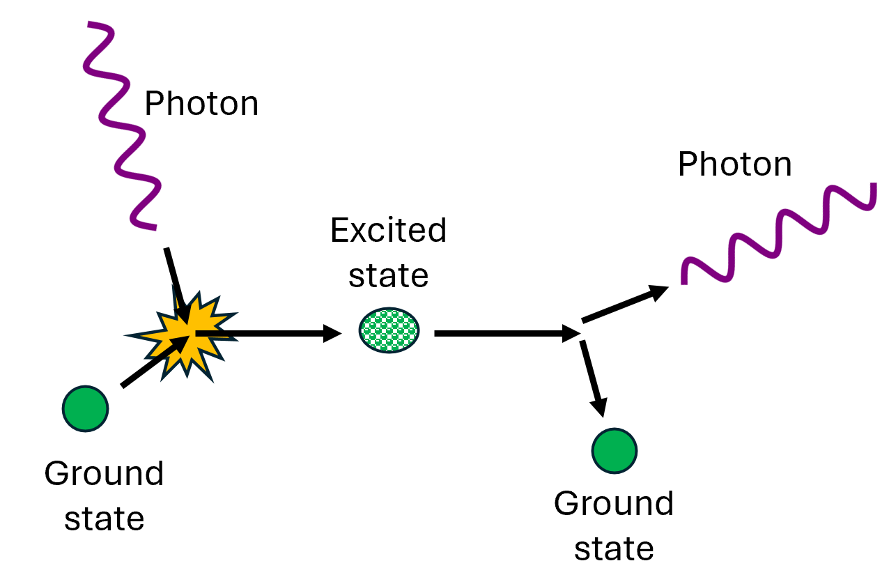
Shining LightFirst, we could shine ultraviolet light (an invisible form of light at slightly higher frequency than visible light) on an atom. If so, we might observe processes such as those sketched in Figure 3: a photon of light strikes the atom in its ground state, and what emerges from the collision is the atom in one of its excited states (possibly plus one or more photons). The simplest possible process involves
- photon + atom in ground state → atom in excited state
The excited atom then reveals itself when, at a later time, short on human scales but often long on atomic scales, it decays back to the ground state,
- atom (excited state) → atom (ground state) + one or more photons
If there’s just one photon in the excited state’s decay, that photon has always the same frequency , which is determined in terms of the energy of the excited state minus the energy of the ground state
where h is Planck’s constant. [A nitpick: this formula applies when the excited atom is stationary, and has a small correction from the fact that the atom will be moving slowly after the decay.]
Atomic CollisionsSecond, we could slam two atoms in the ground state together. If the speed is high enough, one of the two atoms could come out in an excited state, as sketched in Figure 4.
atom (ground state) + atom (ground state) → atom (ground state) + atom (excited state)
Or both atoms could come out in excited states, though not necessarily the same ones. Again, we would learn which excited states were created by looking at the photons emitted when the atoms transition back down to the ground state.
Figure 4: Two atoms collide, and some of the energy of the collision kicks one of them into an excited state. The excited state subsequently decays just as in Figure 3. Could We Excite an Electron?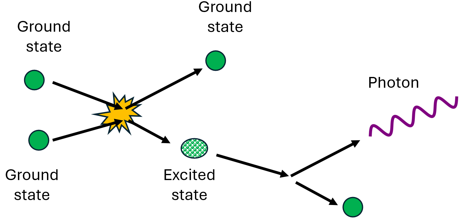
Let’s imagine trying similar tricks just like this on the electron. We could shine high-energy light on the electron, or we could slam electrons together, seeing if we could turn an electron into a muon or a tau.
Shining LightIf a muon is an electron’s excited state, we could shine light waves — gamma-rays this time, as ultraviolet light would not be enough — at electrons, hoping to turn an electron into a muon. Using the notation
- for electron (the minus-sign reflecting its negative electric charge)
- for muon
- for a photon (and for a second photon)
we could try to look for the processes
- ,
possibly plus one or more photons, as shown in Figure 5.
Figure 5: If the electron is the ground state of an object and a muon is an excited state of the same object, then striking an electron with a high-energy photon ought to be able to turn it into a muon (possibly plus additional photons), in analogy to Figure 3.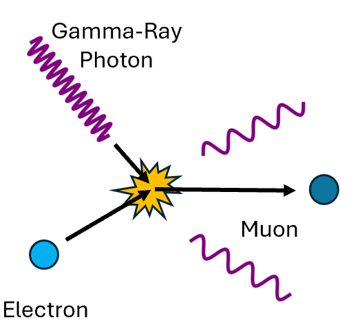
Direct searches for processes like this have been done, and none has ever been seen. Even more significantly, if they were possible, then the following related process (shown in Figure 6) would also be possible
This has been searched for with great effort. Experiments show that no more than one in 2 trillion muons decay this way. The analogous processes for tau’s have never been seen, either.
Figure 6: The decay of a muon to an electron plus a photon has never been observed, despite considerable effort to do so. At best, it is exceedingly rare.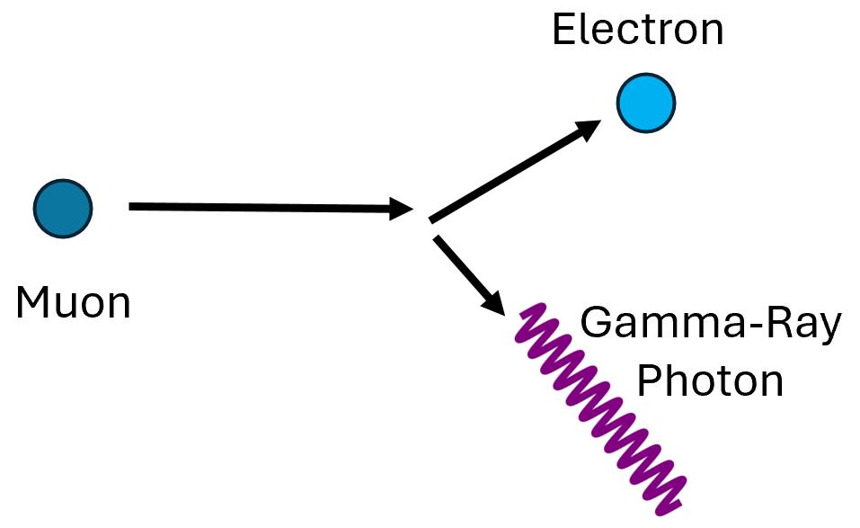
So what? Even though we can’t excite electrons this way, does that really prove that electrons can’t be excited in some other way?
Essentially, it does. The problem is that electrons are electrically charged, and so, if they are made from other, even more elementary objects, then one or more of these objects must also be electrically charged. By its very definition, “having non-zero electric charge” means “able to interact with photons.” It’s virtually impossible to imagine how an electrically charged interior would be unable to absorb photons. So this is an extremely strong mark against the idea.
But just to be sure, let’s try another approach.
Electron-Electron CollisionsWe could also try aiming electrons at each other and seeing what happens when they collide. Just as atomic collisions cause atoms to be excited, we would expect that sufficiently powerful collisions would excite electrons to be muons and taus, and so we should observe processes similar to those in Fig. 4, such as
But again, none of these processes has ever been observed.
Electron-Positron CollisionsIt’s interesting to compare this to what happens in collisions of electrons with the antiparticles of electrons, which are known as positrons and are denoted . In such collisions, we do regularly observe muons and taus appear, as follows
However, we never observe
or anything similar. Only a muon and an anti-muon, or a tau and an anti-tau, are ever created.
Meanwhile, another thing we observe
But clearly photons cannot be excited states of electrons, as photons have zero electric charge and smaller rest mass. So this process has nothing to do with creating an excited state.
Similarly, the processes that create and pairs have a simple interpretation that has nothing to do with electrons having internal structure and excited states. In the process , the electrons are not being kicked into excited states. Instead, the electron and positron are “annihilating” — they are transformed into a disturbance in the electromagnetic field (often called a “virtual photon” — but it is not a particle) — and this disturbance spontaneously transforms into two new particles that are “created” in their stead.
Each of the two new particles is an antiparticle of the other: the muon and the anti-muon , as particle types, are each other’s antiparticles, while photons are their own antiparticles. That’s why electron-positron collisions are just as likely to make photon pairs as to make or . Such annihilation/creation processes occur even for elementary particles, and so their presence gives no evidence supporting the idea of a muon as an excited electron.
We can consider other forms of scattering too, and in none of them do we ever see any of the processes that would be consistent with muons or taus being excited states of electrons. Moreover, all experiments on these particles agree with the math of the Standard Model of particle physics, which is based on the assumption that muons and taus are independent particles from electrons, and are not excited states of the latter.
We can conclude that this excited-electron hypothesis is completely dead. It has been for some decades.
What About Protons?Protons, meanwhile, do have a size. Do the processes mentioned above work for them?
Yes. The first excited state of the proton is called the Delta ; the second is called the . The process
is observed. (In fact this process has a major role to play in the features of cosmic rays, where it causes what is known as the GZK cutoff.) [More easily observed is , which involves a virtual photon and therefore has a similar character.] Also observed is the decay
Scattering processes also create the excited states:
So we see, in experiments, many processes that we would expect to see if the proton is a composite object made of more elementary objects, for which the usual proton is the ground state and the and are excited states.
From these excited states, the size of a proton can be roughly inferred, as explained here.
What About All Those Photons?But what about the fact that even electron-electron collisions often generate photons? Might that be an indication that electrons have excited states?
In other words, even in processes as simple as two electrons that scatter and remain electrons, photons generally appear
- etc.
Why aren’t these indications that electrons are composite? Because, as with the electron-positron annihilation processes discussed earlier, processes like these are expected even for elementary electrons; and predictions for those processes, based on the assumption that electrons are elementary, agree perfectly with data.
So does this mean that electrons definitely are elementary, point-like objects? Not definitely, no. It simply means that if electrons are the ground states of something complex (such as a string, as would potentially be true in string theory), the excited states of that object have far too much rest mass for us to produce them using today’s technology. Someday, collisions may produce them. But for now, all we can say is that in every experiment we can currently perform, electrons appear elementary. So do muons and taus; so do the neutrinos; and so do all six quarks of the Standard Model.
Quick Post: Eyes to the Skies
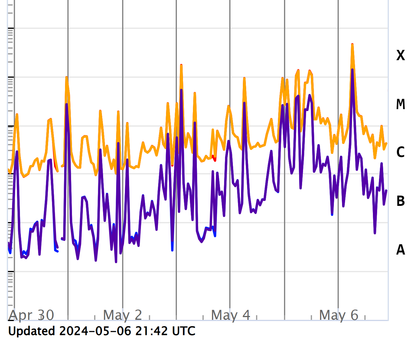
The Sun has been acting up; a certain sunspot has been producing powerful flares. In the past three days, several have reached or almost reached X-class, and one today was an X4.5 flare. (The letter is a measure of energy released by the flare; an X1 flare is ten times more powerful than an M1 class flare, and an X4.5 flare is almost three times more powerful than an X1 flare.)
From the https://www.swpc.noaa.gov/ website
With so much solar activity, it’s possible (though certainly not guaranteed) that one or more coronal mass ejections might strike Earth over the next 48 hours and might generate northern and southern lights (“auroras”). If you’re in a good location and the weather is favorable, you might want to check every now and then to see if the atmosphere is shining at you.
Running Circles Around One Another
Are you sitting or lying down? Perhaps you’re moving around at a walking pace? I probably am. And yet, unless you live in the northeastern US or in southern South America, you and I are moving relative to each other at hundreds of miles per hour.
In Chapter 2 of the book “‘Waves in an Impossible Sea”, I remarked on the this fact. (See below for the relevant passage.) At first glance it might seem puzzling. After all, the distance between your town and my town is constant; it never changes. And yet our relative motion is comparable to or faster than a jet aircraft. How can both of these things be true?
And then there’s another question: if we’re all moving so fast relative to one another, why don’t we feel the motion?
The answer to the second question: It’s the principle of relativity at work. As for the first question: Such is life on a spinning Earth.
In the book, I tried to illustrate how this works using a picture (Figure 2.) But this is one of those cases where an animation is much clearer than a static image. On this new page, I’ve presented animations that I hope will clarify the issue, in case you’re having trouble visualizing it.
Here’s the relevant quote from the book’s Chapter 2, where the principle of relativity is first discussed.
We are oblivious to our own motion, and also to the relative motion between ourselves and our friends in other parts of the world. That relative motion isn’t slow. If people sitting in Boston were to measure carefully, they’d see people standing in Miami as moving at 215 miles (345 km) per hour; meanwhile, those in Miami would perceive their friends in Boston as moving at 215 miles per hour in the opposite direction.
But wait: The distance from Miami to Boston, 1,257 miles (2050 km), never changes, so how can there be relative motion between those two cities? It’s because Bostonians view Miami as moving in a daily circle, one that leaves the distance between the two cities always unchanged—and vice versa.
Details Added to Monday’s Article
A couple of days ago, I posted an article describing how the size of a quantum object, such as a proton or electron, can be measured. This isn’t obvious. For example, scientists say that an electron spreads out and is wave-like, and yet that it has no size. This apparent contradiction needs resolution. While I addressed this puzzle in the book‘s chapter 17, I didn’t do so in detail, and so I wrote this article to fill in the gaps.
Now, in response to a reader’s question, I’ve added a section to the end of the article, entitled “Estimating the Object’s Size From Its Excited States”. There I explain in more detail how one goes from simple measurements, which confirm that a proton’s size isn’t zero, to an actual estimate of a proton’s size. The discussion is a little more technical than the rest of the article; you will probably need first-year physics to follow it. But I hope that some readers will find it useful!
How Do You Measure a Quantum Object’s Size?
Quantum physics is certainly confusing.
- On the one hand, electrons are wave-like and can be quite spread out; in fact, as I’ve emphasized in my book and in a recent blog post, a stationary electron is a spread-out standing wave. (I’ve even argued that these “elementary particles” should really be called “wavicles” [a term from the 1920s].)
- On the other hand, scientists say that electrons have no size — or at least, if they have a size, it’s too small to be measured using current technology. They are often described as “point particles.”
How can both these things be true?
Well, to clarify this, let’s look at objects that do have an intrinsic size, such as protons and neutrons. How are their sizes actually determined? While this question is addressed in the book’s Chapter 17 (see Figure 40 and surrounding text, and footnote 2), I didn’t go into much detail there.
To supplement what’s in the book, I have written a webpage that outlines two classic methods that are used to measure the intrinsic size of a proton, or of any ultra-microscopic object.
When these same methods are used on electrons, one finds no evidence of any finite size, and so one concludes that their intrinsic size (if any) is too small to measure.
Why a Wave Function Can’t Hurt You
In recent talks at physics departments about my book, I have emphasized that the elementary “particles” of nature — electrons, photons, quarks and so on — are really little waves (or, to borrow a term that was suggested by Sir Arthur Eddington in the 1920s, “wavicles”.) But this notion inevitably generates confusion. That’s because of another wavy concept that arises in “quantum mechanics” —the quantum physics of the 1920s, taught to every physics student. That concept is Erwin Schrödinger’s famous “wave function”.
It’s natural to guess that wave functions and wavicles are roughly the same. In fact, however, they are generally unrelated.
Wavicles Versus Wave FunctionsBefore quantum physics came along, field theory was already used to predict the behavior of ordinary waves in ordinary settings. Field theory is useful for sound waves in air, seismic waves in rock, and waves on water.
Quantum field theory, the quantum physics that arose out of the 1940s and 1950s, adds something new: it tells us that waves in quantum fields are made from wavicles, the gentlest possible waves. A photon, for instance, is a wavicle of light — the dimmest possible flash of light.
By contrast, a wave function describes a system of objects operating according to quantum physics. Importantly, it’s not one wave function per object — it’s one wave function per system of interacting objects. That’s true whether the objects in the system are particles in motion, or something as simple as particles that cannot move, or something as complex as fields and their wavicles.
One of the points I like to make, to draw the distinction between these two types of waves in quantum physics, is this:
- Wavicles can hurt you.
- Wave functions cannot.
Daniel Whiteson, the well-known Large Hadron Collider physicist, podcaster and popular science writer, liked this phrasing so much that he quoted the second half on X/Twitter. Immediately there were protests. One person wrote “Everything that has ever hurt anyone was in truth a wave function.” Another posted a video of an unfortunate incident involving the collision between a baseball and a batter, and said: “the wave function of this baseball disagrees.”
It’s completely understandable why there’s widespread muddlement about this. We have two classes of waves floating around in quantum physics, and both of them are inherently confusing. My aim today is to make it clear why a wave function couldn’t hurt a fly, a cat, or even a particle.
The Basic ConceptsWavicles, such as photons or electrons, are real objects. X-rays are a form of light, and are made of photons — wavicles of light. A strong beam of X-ray photons can hurt you. The photons travel across three-dimensional space carrying energy and momentum; they can strike your body, damage your DNA, and thereby cause you to develop cancer.
The wave function associated with the X-ray beam, however, is not an object. All it does is describe the beam and its possible futures. It tells us what the beam’s energy may be, but it doesn’t have any energy, and cannot inflict the beam’s energy on anything else. The wave function tells us where the beam may go, but itself goes nowhere. Though it describes a beam as it crosses ordinary three-dimensional space, the wave function does not itself exist in three-dimensional space.
In fact, if the X-ray beam is interacting with your body, then the X-ray beam cannot be said to have its own wave function. Instead, there is only one wave function — one that describes the beam of photons, your atoms, and the interactions between your atoms and the photons.
More generally, if a bunch of objects interact with each other,the multiple interacting objects form a single indivisible system, and a single wave function must describe it. The individual objects do not have separate wave functions.
Schrödinger’s CatThis point is already illustrated by Schrödinger’s famous (albeit unrealistic) example of the cat in a box that is both dead and alive. The box contains a radioactive atom which will, via a quantum process, eventually “decay” [i.e. transform itself into a new type of atom, releasing a subatomic particle in the process], but may or may not have done so yet. If and when the atom does decay, it triggers the poisoning of the cat. The cat’s survival or demise thus depends on a quantum effect, and it becomes a party to a quantum phenomenon.
It would be a mistake to say that “the atom has a wave function” (or even worse, that “the atom is a wave function”) and that this wave function can kill the cat. To do so would miss Schrödinger’s point. Instead, the wave function includes the atom, the killing device, and the cat.
Initially, when the box is closed, the three are independent of one another, and so they have a relatively simple wave function which one may crudely sketch as
- Wave Function = (atom undecayed) x (device off) x (cat alive)
This wave function represents our certainty that the atom has not yet decayed, the murder weapon has not been triggered, and the cat is still alive.
But this initial wave function immediately begins evolving into a more complicated form, one which depends on two time-varying complex numbers C and D, with |C|2 + |D|2 = 1:
- Wave Function = C(t) x (atom undecayed) x (device off) x (cat alive) + D(t) x (atom decayed) x (device on) x (cat dead)
The wave function is now a sum of two “branches” which describe two distinct possibilities, and assigns them probabilities |C|2 and |D|2, the former gradually decreasing and the latter gradually increasing. [Note these two branches are added together in the wave function; its branches cannot be rearranged into wave functions for the atom, device and cat separately, nor can the two branches ever be separated from one another.]
In no sense has the wave function killed the cat; in one of its branches the cat is dead, but the other branch describes a live cat. And in no sense did the “wave function of the atom” or “of the device” kill the cat, because no such wave functions are well-defined in this interacting system.
A More Explicit ExampleLet’s now look at an example, similar to the cat but more concrete, and easier to think about and draw.
Let’s take two particles [not wavicles] A and B. These particles travel only in a one-dimensional line, instead of in three-dimensional space.
Initially, particle B is roughly stationary and particle A comes flying toward it. There are two possible outcomes.
- There is a 30% probability that A passes right by B without affecting it, in which case B simply says “hi” as A goes by.
- There is a 70% probability that A strikes B head-on and bounces off of it, in which case B, recoiling from the blow, says “ow”.
In the second case, we may indeed say that A “hurts” B — at least in the sense of causing B to recoil suddenly.
The Classical ProbabilitiesBefore we answer quantum questions, let’s first think about how one might describe this situation in a world without quantum physics. There are several ways of depicting what may happen.
Motion in One-Dimensional Physical SpaceWe could describe how the particles move within their one-dimensional universe, using arrows to illustrate their motions over time. In the figure below, I show both the “hi” possibility and the “ow” possibility.
Figure 1: (Top) With 30% probability, the Hi case: A (in blue) passes by B without interacting with it. (Bottom) With 70% probability, the Ow case: A strikes B, following which A rebounds and B recoils.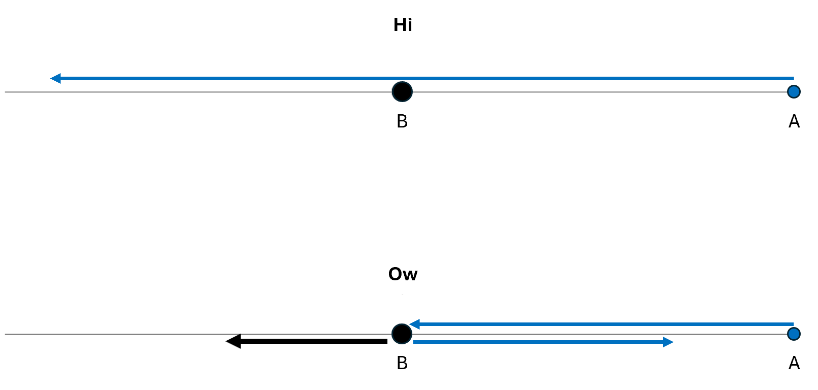
Or, using an animation, we can show the time-dependence more explicitly and more clearly. In the second case, I’ve assumed that B has more mass than A, so it recoils more slowly from the blow than does A.
Figure 2: Animation of Fig. 1, showing the Hi case in which A passes B, and the Ow case where A strikes B. Motion in the Two-Dimensional Space of Possibilities
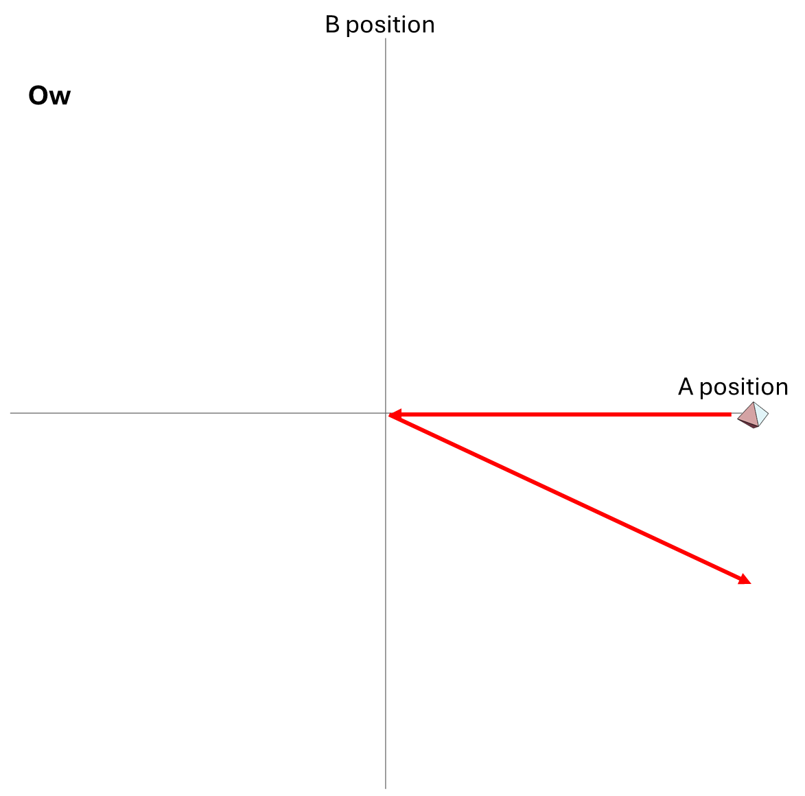
But we could also describe how the particles move as a system in their two-dimensional space of possibilities. Each point in that space tells us both where A is and where B is; the point’s location along the horizontal axis gives A’s position, and its location along the vertical axis gives B’s position. At each moment, the system is at one point in that space; over time, as A and B change their positions, the location of the system in that two-dimensional space also changes.
The motion of the system for the Hi and Ow cases is shown in Fig. 3. It has exactly the same information as Fig. 1, though depicted differently and somewhat more precisely. Instead of following the two dots that correspond to the two particles as they move in one dimension, we now depict the whole system as a single diamond that tells us where both particles are located.
In the first part of Fig. 3, we see that B’s position is at the center of the space, and remains there, while A’s position goes from the far right to the far left; compare to Fig. 1. In the second part of Fig. 3, A and B collide at the center, following which A moves to positive position, B moves to negative position, and correspondingly, within its space of possibilities, the system as a whole moves down and to the right.
Figure 3: How the A/B system moves through the space of possibilities. (Top) In the Hi case, A moves while B remains fixed at its central position. (Botttom) The Ow case is the same as the Hi case until A’s position reaches B’s position at the center; a collision then causes A to reverse course to a positive position, while B is driven to a negative position (which is downward in this graph.) The system as a whole thus moves down and to the right in the space of possibilities.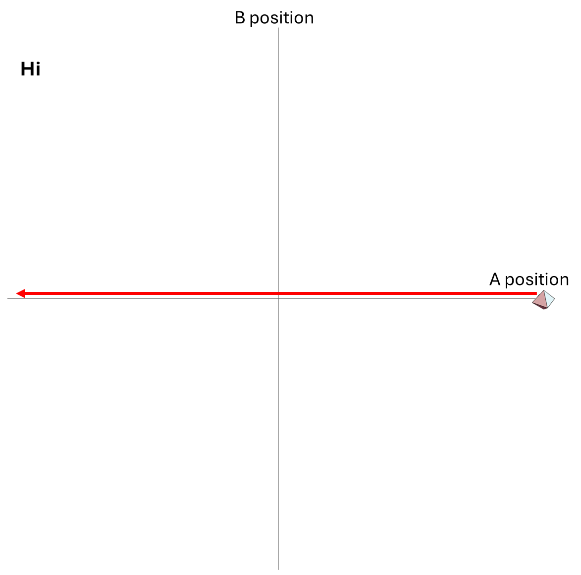
And finally, let’s look at an animation in the two-dimensional space of possibilities. Compare this to Fig. 3, and then to Fig. 2, noting that it has the same information.
Figure 4: Animation of Figure 3, showing (top) the Hi case in which A passes B and (bottom) the Ow case where A strikes B.
In Fig. 4, we see that
- the system as a whole is represented as a single moving point in the space of possibilities
- each of the two futures for the system are represented as separate time-dependent paths across the space of possibilities
Now, what if the system is described using quantum physics? What’s up with the system’s wave function?
As noted, we do not have a wave function for particle A and a separate wave function for particle B, and so we do not have a collision of two wave functions. Instead, we have a single wave function for the A/B system, one which describes the collision of the two particles and the aftermath thereof.
It is impossible to depict the wave function using the one-dimensional universe that the particles live in. The wave function itself only exists in the space of possibilities. So in quantum physics, there are no analogues to Figs. 1 and 2.
Meanwhile, although we can depict the wave function at any one moment in the two dimensional space, we cannot simply use arrows to depict how it changes over time. This is because we cannot view the “Hi” and “Ow” cases as distinct, and as something we can draw in two separate figures, as we did in Figs. 3 and 4. In quantum physics, we have to view both possibilities as described by the same wave function; they are not distinct outcomes.
The only option we have is to do an animation in the two-dimensional space of possibilities, somewhat similar to Fig. 4, but without separating the Hi and Ow outcomes. There’s just one wave function that shows both the “Hi” and “Ow” cases together. The square of this wave function, which gives the probabilities for the system’s possible futures, is sketched in Fig. 5.
[Note that what is shown is merely a sketch! It is not the true wave function, which requires a complete solution of Schrödinger’s wave equation. While the solution is well known, it is tricky to get all the details of the math exactly right, and I haven’t had the time. I’ll try to add the complete and correct solution at a later date.]
Compare Fig. 5 with Fig. 4, recalling that the probability of the Hi case is 30% and the probability of the Ow case is 70%. Both possibilities appear in the wave function, with the branch corresponding to the Ow case carrying larger weight than the branch corresponding to the Hi case.
Figure 5: A rough sketch of what the square of the wave function of the A/B system looks like; small-scale details are not modeled correctly. Note both Hi and Ow possibilities, and their relative probabilities, appear in the wave function. Compare with Fig. 4 and with the example of Schrödinger’s cat.
In contrast to Fig. 4, the key differences are that
- the system is no longer represented as a point in the space of possibilities, but instead as a (broadened) set of possibilities
- the wave function is complicated during the collision, and develops two distinct branches only after the collision
- all possible futures for the system exist within the same wave function
- this has the consequence that distinct future possibilities of the system could potentially affect each other at a later time — a concept which makes no sense in non-quantum physics
- the probabilities of those distinct futures are given by the relative sizes of the wave function within the two branches.
Notice that even though particle A has a 70% probability of “hurting” B, the wave function itself does not, and cannot, “hurt” B. It just describes what may happen; it contains both A and B, and describes both the possibility of Hi and Ow. The wave function isn’t a part of the A/B system, and doesn’t participate in its activities. Instead, it exists outside the system, as a means for understanding that system’s behavior.
Summing UpA system has a wave function, but individual objects in the system do not have wave functions. That’s the key point.
To be fair, it is true that when objects or groups of objects in a system interact weakly enough, we may imagine the system’s full wave function as though it were a simple combination of wave functions for each object or group of objects. That is true of the initial Schrödinger cat wave function, which is a product of separate factors for the atom, device and cat, and is also true of the wave function in Fig. 5 before the collision of A and B. But once significant interactions occur, this is no longer the case, as we see in the later-stage Schrödinger cat wave function and in Fig. 5 after the collision.
A wave function expresses how the overall system moves through the full space of its possibilities, and grows ever more complex when there are many possible paths for a system to take. This is completely unrelated to wavicles, which are objects that move through physical space and create physical phenomena, forming parts of a system that itself is described by a wave function.
A Final Note on Wave FunctionsAs a final comment: I’ve given this simple example because it’s one of the very few that one can draw start to finish.
Wave functions of systems with just one particle are misleading, because they make it easy to imagine that there is one wave function per particle. But with more than one particle, the only wave functions that can easily be depicted are those of two particles moving in one dimension, such as the one I have given you. Such examples offer a unique opportunity to clarify what a wave function is and isn’t, and it’s therefore crucial to appreciate them.
Any wave function more complicated than this becomes impossible to draw. Here are some things to consider.
- I have only drawn the square of the wave function in Fig. 5. The full wave function is a complex function (i.e. a complex number at each point in the space of possibilities), and the contour plot I have used in Fig. 5 could only be used to draw its real part, its imaginary part, or its square. Thus even in this simple situation with a two-dimensional space of possibilities, the full wave function cannot easily be represented.
- If we had four particles moving in one dimension instead of two, with positions x1, x2, x3 and x4 respectively, then the wave function would be a function of the four-dimensional space of possibilities, with coordinates x1, x2, x3, x4 . [The square of the wave function at each point in that space tells us the probability that particle 1 is at position x1, particle 2 is at position x2, and similarly for 3 and 4.] A function in four dimensions can be handled using math, but is impossible to draw.
- If we had two particles moving in three dimensions, the first with position x1, y1, z1, and the second with position x2, y2, z2, the space of possibilities would be six-dimensional — x1, y1, z1, x2, y2, z2 . Again, this cannot be drawn.
These difficulties explain why one almost never sees a proper discussion of wave functions of complicated systems, and why wave functions of fields are almost never described and are never depicted.
Speaking Today in Seattle, Tomorrow near Portland
A quick reminder, to those in the northwest’s big cities, that I will be giving two talks about my book in the next 48 hours:
- At Seattle’s Town Hall, tonight (April 17th) at 7:30 pm.
- Near Portland, at the Cedar Hills branch of Powell’s Books, tomorrow (April 18th) at 7:00 pm.
Hope to see some of you there! (You can keep track of my speaking events at my events page.)
Why The Higgs Field is Nothing Like Molasses, Soup, or a Crowd
The idea that a field could be responsible for the masses of particles (specifically the masses of photon-like [“spin-one”] particles) was proposed in several papers in 1964. They included one by Peter Higgs, one by Robert Brout and Francois Englert, and one, slightly later but independent, by Gerald Guralnik, C. Richard Hagen, and Tom Kibble. This general idea was then incorporated into a specific theory of the real world’s particles; this was accomplished in 1967-1968 in two papers, one written by Steven Weinberg and one by Abdus Salam. The bare bones of this “Standard Model of Particle Physics” was finally confirmed experimentally in 2012.
How precisely can mass come from a field? There’s a short answer to this question, invented a couple of decades ago. It’s the kind of answer that serves if time is short and attention spans are limited; it is intended to sound plausible, even though the person delivering the “explanation” knows that it is wrong. In my recent book, I called this type of little lie, a compromise that physicists sometimes have to make between giving no answer and giving a correct but long answer, a “phib” — a physics fib. Phibs are usually harmless, as long as people don’t take them seriously. But the Higgs field’s phib is particularly problematic.
The Higgs PhibThe Higgs phib comes in various forms. Here’s a particularly short one:
There’s this substance, like a soup, that fills the universe; that’s the Higgs field. As objects move through it, the soup slows them down, and that’s how they get mass.
Some variants replace the soup with other thick substances, or even imagine the field as though it were a crowd of people.
How bad is this phib, really? Well, here’s the problem with it. This phib violates several basic laws of physics. These include foundational laws that have had a profound impact on human culture and are the first ones taught in any physics class. It also badly misrepresents what a field is and what it can do. As a result, taking the phib seriously makes it literally impossible to understand the universe, or even daily human experience, in a coherent way. It’s a pedagogical step backwards, not forwards.
What’s Wrong With The Higgs PhibSo here are my seven favorite reasons to put a flashing red warning sign next to any presentation of the Higgs phib.
1. Against The Principle of RelativityThe phib brazenly violates the principle of relativity — both Galileo’s original version and Einstein’s updates to it. That principle, the oldest law of physics that has never been revised, says that if your motion is steady and you are in a closed room, no experiment can tell you your speed, your direction of motion, or even whether you are in motion at all. The phib directly contradicts this principle. It claims that
- if an object moves, the Higgs field affects it by slowing it down, while
- if it doesn’t move, the Higgs field does nothing to it.
But if that were true, the action of the Higgs field could easily allow you to distinguish steady motion from being stationary, and the principle of relativity would be false.
2. Against Newton’s First Law of MotionThe phib violates Newton’s first law of motion — that an object in motion not acted on by any force will remain in steady motion. If the Higgs field slowed things down, it could only do so, according to this law, by exerting a force.
But Newton, in predicting the motions of the planets, assumed that the only force acting on the planets was that of gravity. If the Higgs field exerted an additional force on the planets simply because they have mass (or because it was giving them mass), Newton’s methods for predicting planetary motions would have failed.
Worse, the slowing from the Higgs field would have acted like friction over billions of years, and would by now have caused the Earth to slow down and spiral into the Sun.
3. Against Newton’s Second Law of MotionThe phib also violates Newton’s second law of motion, by completely misrepresenting what mass is. It makes it seem as though mass makes motion difficult, or at least has something to do with inhibiting motion. But this is wrong.
As Newton’s second law states, mass is something that inhibits changes in motion. It does not inhibit motion, or cause things to slow down, or arise from things being slowed down. Mass is the property that makes it hard both to speed something up and to slow it down. It makes it harder to throw a lead ball compared to a plastic one, and it also makes the lead ball harder to catch bare-handed than a plastic one. It also makes it difficult to change something’s direction.
To say this another way, Newton’s second law F=ma says that to make a change in an object’s motion (an acceleration a) requires a force (F); the larger the object’s mass (m), the larger the required force must be. Notice that it does not have anything to say about an object’s motion (its velocity v).
To suggest that mass has to do with motion, and not with change in motion, is to suggest that Newton’s law should be F=mv — which, in fact, many pre-Newtonian physicists once believed. Let’s not let a phib throw us back to the misguided science of the Middle Ages!
4. Not a Universal Mass-GiverThe phib implies that the Higgs field gives mass to all objects with mass, causing all of them to slow down. After all, if there were a universal “soup” found everywhere, then every object would encounter it. If it were true that the Higgs field acted on all objects in the same way — “universally”, similar to gravity, which pulls on all objects — then every object in our world would get its mass from the Higgs field.
But in fact, the Higgs field only generates the masses of the known elementary particles. More complex particles such as protons and neutrons — and therefore the atoms, molecules, humans and planets that contain them — get most of their mass in another way. The phib, therefore, can’t be right about how the Higgs field does its job.
5. Not Like a SubstanceAs is true of all fields, the Higgs field is not like a substance, in contrast to soup, molasses, or a crowd. It has no density or materiality, as soup would have. Instead, the Higgs field (like any field!) is more like a property of a substance.
As an analogue, consider air pressure (which is itself an example of an ordinary field.) Air is a substance; it is made of molecules, and has density and weight. But air’s pressure is not a thing; it is a property of air, , and is not itself a substance. Pressure has no density or weight, and is not made from anything. It just tells you what the molecules of air are doing.
The Higgs field is much more like air pressure than it is like air itself. It simply is not a substance, despite what the phib suggests.
6. Not Filling the UniverseThe Higgs field does not “fill” the universe any more than pressure fills the atmosphere. Pressure is found throughout the atmosphere, yes, but it is not what makes the atmosphere full. Air is what constitutes the atmosphere, and is the only thing that can be said, in any sense, to fill it.
While a substance could indeed make the universe more full than it would otherwise be, a field of the universe is not a substance. Like the magnetic field or any other cosmic field, the Higgs field exists everywhere — but the universe would be just as empty (and just as full) if the Higgs field did not exist.
7. Not Merely By Its PresenceFinally, the phib doesn’t mention the thing that makes the Higgs field special, and that actually allows it to affect the masses of particles. This is not merely that it is present everywhere across the universe, but that it is, in a sense, “on.” To give you a sense of what this might mean, consider the wind.
On a day with a steady breeze, we can all feel the wind. But even when the wind is calm, physicists would say that the wind exists, though it is inactive. In the language I’m using here, I would say that the wind is something that can always be measured — it always exists — but
- on a calm day it is “off” or “zero”, while
- on a day with a steady breeze, it is “on” or “non-zero”.
In other words, the wind is always present, whether it is calm or steady; it can always be measured.
In rough analogy, the Higgs field, though switched on in our universe, might in principle have been off. A switched-off Higgs field would not give mass to anything. The Higgs field affects the masses of elementary particles in our universe only because, in addition to being present, it is on. (Physicists would say it has a “non-zero average value” or a “non-zero vacuum expectation value”)
Why is it on? Great question. From the theoretical point of view, it could have been either on or off, and we don’t know why the universe arranged for the former.
Beyond the Higgs PhibI don’t think we can really view a phib with so many issues as an acceptable pseudo-explanation. It causes more problems and confusions than it resolves.
But I wish it were as easy to replace the Higgs phib as it is to criticize it. No equally short story can do the job. If such a brief tale were easy to imagine, someone would have invented it by now.
Some years ago, I found a way to explain how the Higgs field works that is non-technical and yet correct — one that I would be happy to present to my professional physics colleagues without apology or embarrassment. (In fact, I did just that in my recent talks at the physics departments at Vanderbilt and Irvine.) Although I tried delivering it to non-experts in an hour-long talk, I found that it just doesn’t fit. But it did fit quite well in a course for non-experts, in which I had several hours to lay out the basics of particle physics before addressing the Higgs field’s role.
That experience motivated me to write a book that contains this explanation. It isn’t brief, and it’s not a light read — the universe is subtle, and I didn’t want to water the explanation down. But it does deliver what it promises. It first carefully explains what “elementary particles” and fields really are [here’s more about fields] and what it means for such a “particle” to have mass. Then it gives the explanation of the Higgs field’s effects — to the extent we understand them. (Readers of the book are welcome to ask me questions about its content; I am collecting Q&A and providing additional resources for readers on this part of the website.)
A somewhat more technical explanation of how the Higgs field works is given elsewhere on this website: check out this series of pages followed by this second series, with additional technical information available in this third series. These pages do not constitute a light read either! But if you are comfortable with first-year university math and physics, you should be able to follow them. Ask questions as need be.
Between the book, the above-mentioned series of webpages, and my answers to your questions, I hope that most readers who want to know more about the Higgs field can find the explanation that best fits their interests and background.
Update to the Higgs FAQ
Although I’ve been slowly revising the Higgs FAQ 2.0, this seemed an appropriate time to bring the Higgs FAQ on this website fully into the 2020’s. You will find the Higgs FAQ 3.0 here; it explains the basics of the Higgs boson and Higgs field, along with some of the wider context.
For deeper explanations of the Higgs field:
- if you are comfortable with math, you can find this series of pages useful (but you will probably to read this series first.)
- if you would prefer to avoid the math, a full and accurate conceptual explanation of the Higgs field is given in my book.
Events: this week I am speaking Tuesday in Berkeley, CA; Wednesday in Seattle, WA (at Town Hall); and Thursday outside of Portland, OR (at the Powell’s bookstore in Cedar Hills). Click here for more details.
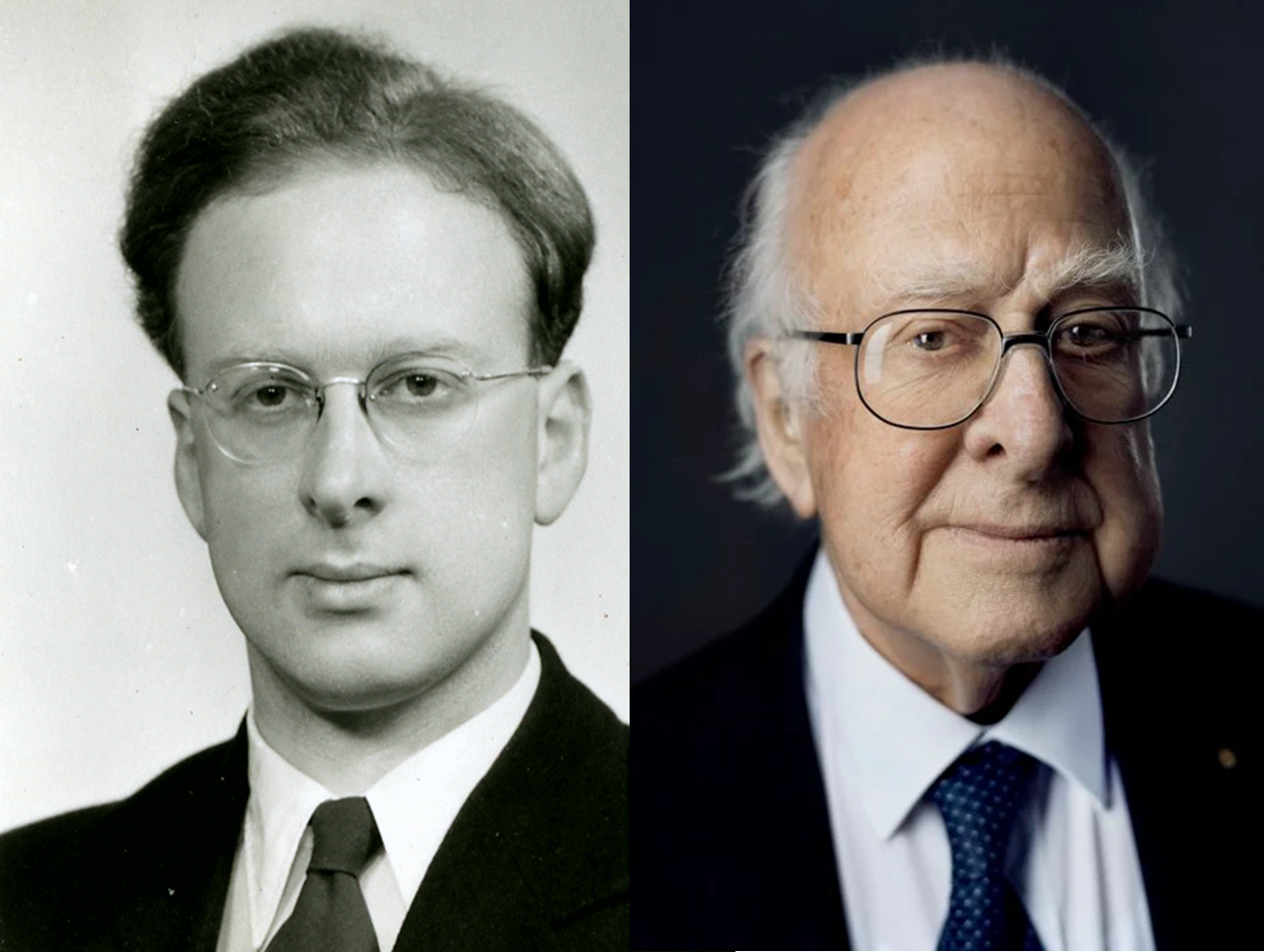
Peter Higgs versus the “God Particle”
The particle physics community is mourning the passing of Peter Higgs, the influential theoretical physicist and 2013 Nobel Prize laureate. Higgs actually wrote very few papers in his career, but he made them count.
It’s widely known that Higgs deeply disapproved of the term “God Particle”. That’s the nickname that has been given to the type of particle (the “Higgs boson”) whose existence he proposed. But what’s not as widely appreciated is why he disliked it, as do most other scientists I know.
It’s true that Higgs himself was an atheist. Still, no matter what your views on such subjects, it might bother you that the notion of a “God Particle” emerged neither from science nor from religion, and could easily be viewed as disrespectful to both of them. Instead, it arose out of marketing and advertising in the publishing industry, and it survives due to another industry: the news media.
But there’s something else more profound — something quite sad, really. The nickname puts the emphasis entirely in the wrong place. It largely obscures what Higgs (and his colleagues/competitors) actually accomplished, and why they are famous among scientists.
Let me ask you this. Imagine a type of particle that
- once created, vanishes in a billionth of a trillionth of a second,
- is not found naturally on Earth, nor anywhere in the universe for billions of years,
- has no influence on daily life — in fact it has never had any direct impact on the human species — and
- only was discovered when humans started making examples artificially.
This doesn’t seem very God-like to me. What do you think?
Perhaps this does seem spiritual or divine to you, and in that case, by all means call the “Higgs boson” the “God Particle”. But otherwise, you might want to consider alternatives.
For most humans, and even for most professional physicists, the only importance of the Higgs boson is this: it gives us insight into the Higgs field. This field
- exists everywhere, including within the Earth and within every human body,
- has existed throughout the history of the known universe,
- has been reliably constant and steady since the earliest moments of the Big Bang, and
- is crucial for the existence of atoms, and therefore for the existence of Earth and all its life;
It may even be capable of bringing about the universe’s destruction, someday in the distant future. So if you’re going to assign some divinity to Higgs’ insights, this is really where it belongs.
In short, what’s truly consequential in Higgs’ work (and that of others who had the same basic idea: Robert Brout and Francois Englert, and Gerald Guralnik, C. Richard Hagen and Tom Kibble) is the Higgs field. Your life depends upon the existence and stability of this field. The discovery in 2012 of the Higgs boson was important because it proved that the Higgs field really exists in nature. Study of this type of particle continues at the Large Hadron Collider, not because we are fascinated by the particle per se, but because measuring its properties is the most effective way for us to learn more about the all-important Higgs field.
Professor Higgs helped reveal one of the universe’s great secrets, and we owe him a great deal. I personally feel that we would honor his legacy, in a way that would have pleased him, through better explanations of what he achieved — ones that clarify how he earned a place in scientists’ Hall of Fame for eternity.
Star Power
A quick note today, as I am flying to Los Angeles in preparation for
- A book talk 4/10 at Vroman’s Bookstore in Pasadena, CA
- A colloquium-style talk 4/11 (related to the book) at the University of Irvine physics department
and other events next week.
I hope many of you were able, as I was, to witness the total solar eclipse yesterday. This was the third I’ve seen, and each one is different; the corona, prominences, stars, planets, and sky color all vary greatly, as do the sounds of animals. (I have written about my adventures going to my first one back in 1999; yesterday was a lot easier.)
Finally, of course, the physics world is mourning the loss of Peter Higgs. Back in 1964, Higgs proposed the particle known as the Higgs boson, as a consequence of what we often call the Higgs field. (Note that the field was also proposed, at the same time, by Robert Brout and Francois Englert.) Much is being written about Higgs today, and I’ll leave that to the professional journalists. But if you want to know what Higgs actually did (rather than the pseudo-descriptions that you’ll find in the press) then you have come to the right place. More on that later in the week.
DESI Shakes Up the Universe
It’s always fun and interesting when a measurement of an important quantity shows a hint of something unexpected. If yesterday’s results from DESI (the Dark Energy Spectroscopic Instrument) were to hold up to scrutiny, it would be very big news. We may well find out within a year or two, when DESI’s data set triples in size.
The phrase “Dark Energy” is shorthand for “the energy-density and negative pressure of empty space”. This quantity was found to be non-zero back in 1998. But there’s been insufficient data to determine whether it has been constant over the history of the universe. Yesterday’s results from DESI suggest it might not be constant; perhaps the amount of dark energy has varied over time.
If so, this would invalidate scientists’ simplest viable model for the universe, the benchmark known as the “Standard Model of Cosmology” (not to be confused with the “Standard Model of Particle Physics.”, which is something else altogether.) In cosmology’s standard model, nicknamed ΛCDM, there is a constant amount of dark energy [Λ], along with a certain amount of relatively slow-moving (i.e. “cold”) dark matter [CDM] (meaning some kind of stuff that gravitates, but doesn’t shine in any way). All this is accompanied by a little bit of ordinary stuff, out of which familiar objects like planets and bloggers are made.
While ΛCDM agrees with most existing data, it’s crude, and may well be too simple. Perhaps it requires a small tweak. Or perhaps it requires a larger adjustment. We have already had a puzzle for several years, called the “Hubble tension”, concerning the so-called Hubble constant, which is a measure of how quickly the universe has been expanding over time. Measurements of the Hubble constant can be made by studying the nearby universe today; others can be made using views of the universe’s more distant past; and the two classes of measurements disagree by a few percent. This disagreement suggests that maybe there’s an important detail missing from the standard picture of the cosmos’s history.
Now, perhaps DESI has seen a sign of something else in ΛCDM breaking down… specifically the idea of a constant Λ. (At the moment, I know of no obvious relation between DESI’s results and the Hubble tension.) But it’s too early to say for sure; in fact, even if DESI’s results hold up over time, it might be that there are multiple interpretations of their results.
An aside, in answer to a common question: Is the whole concept of the Big Bang at risk? I doubt that very much. The discrepancies are only a few percent. They seem enough to potentially challenge important details, but nowhere near enough to undermine the whole story.
There are a number of murky elements here; in particular, DESI’s data is still limited enough that one’s interpretations of their results depends on one’s assumptions. (There’s also a story here involving the masses of neutrinos, which also depends upon one’s assumptions.) I don’t understand all the issues yet, but I’ll try to wrap my head around them soon, and report back to you. It happens that I’m in the middle of some travel for talks about my book (in CA, WA and OR; you can check my event page) so it may take me a little while, I’m afraid. In the meantime, you might want to read about the Baryon Acoustic Oscillations [BAO] that lie at the heart of DESI’s measurements.
[Postscript: I guess Nature liked my title and decided to shake up New Jersey today… as felt today even in Massachusetts.]
Speaking at Harvard Tonight at 6pm
A reminder: tonight (April 3) at 6pm I’ll be giving a public lecture about my book, along with a Q&A in conversation with Greg Kestin, at Harvard University’s Science Center. It’s free, though they request an RSVP. More details are here. Please spread the word! (Next event in Pasadena, CA on April 10th.)
Total Eclipse a Week Away
I hope that a number of you will be able to see the total solar eclipse next Monday, April 8th. I have written about my adventures taking in a similar eclipse in 1999, an event which had a profound impact on me. Perhaps my experience might give you some things to think about that go well beyond the mere scientific.
Meanwhile, for those who can only see a partial solar eclipse that day, there’s still something really cool (and very poorly appreciated!) that you can do that cannot be done on an ordinary day! Namely, you can easily estimate the size of the Moon, and then quickly go on to estimate how far away it is. This is daylight astronomy at its best!
Side note for those in the Boston area: I’m speaking about my new book at Harvard on Wednesday April 3rd.
For Subscribers: Reminder of Book Discount, and Upcoming Talks
You're currently a free subscriber. Upgrade your subscription to get access to the rest of this post and other paid-subscriber only content.
Upgrade subscriptionSpeaking in Nashville, Cambridge and the West Coast
I’m beginning a period of travel and public speaking, so new posts may be a bit limited for a time. (Meanwhile, explore this site’s other offerings!) Tomorrow, Thursday March 28th, I’ll be in Nashville, at Vanderbilt University’s department of physics and astronomy, giving a talk (at 4 pm) about the subjects covered in my recent book. Next, on Wednesday April 3rd (6 pm) I’ll be in Cambridge, Massachusetts, giving a public talk about the book at the Harvard Science Center, as organized by the Harvard Bookstore (the wonderful independent book store located right in Harvard Square.) [Free, but RSVP.]
Then I’ll be on the west coast for a couple of weeks; if you live out there, check out this site’s upcoming-events page. And if you can’t attend any of these events, you can always listen to the recent podcasts that I’ve been on, with Sean Carroll (here) and with Daniel Whiteson (part 1 and part 2.)
More physics coming soon!
How To Make A Standing Wave Without Edges
I recently pointed out that there are unfamiliar types of standing waves that violate the rules of the standing waves that we most often encounter in life (typically through musical instruments, or when playing with ropes and Slinkys) and in school (typically in a first-year physics class.) I’ve given you some animations here and here, along with some verbal explanation, that show how the two types of standing waves behave.
Today I’ll show you what lies “under the hood” — and how you yourself could make these unfamiliar standing waves with a perfectly ordinary physical system. (Another example, along with the relevance of this whole subject to the Higgs field, is discussed in chapter 20 of the book.)
Strings, Balls and SpringsIt’s a famous fact that an ordinary string bears a close resemblance to a set of balls connected by springs — their waves are the same, as long as the wave’s shape varies slowly compared to the distance between the balls.
Figure 1: (Top) A length of string. (Bottom) A set of balls connected by springs. The vertical waves of the ball-spring system are similar to the vertical waves on the string; see Figure 2.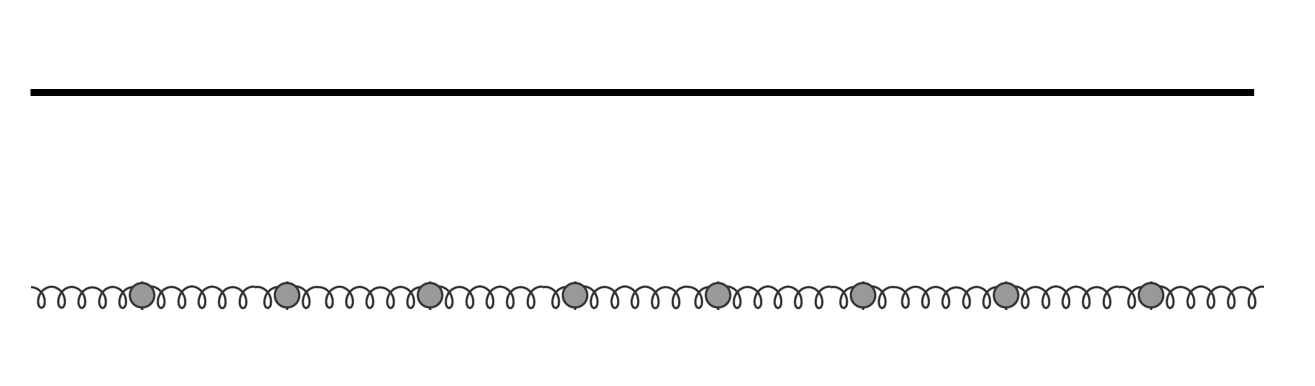
The string remains continuous, rather than fragmenting into pieces, because of its internal atomic forces. Similarly, in the ball-spring system, continuity is assured by the springs, which prevent neighboring balls from moving too far apart.
Both systems have familiar standing waves like those on a guitar string, but only if their ends are attached and fixed to something. The most familiar standing wave, shown for each of the two systems, is displayed below.
Figure 2: The classic standing wave for the string and for the the ball-spring system A Different Set of Balls and Springs
Figure 3 shows a different system of balls and springs, unlike a guitar string. Here, the two sets of springs have distinct roles to play.
Figure 3: A set of balls connected to each other by horizontal springs and to the ground by vertical springs. The waves of this system are less familiar.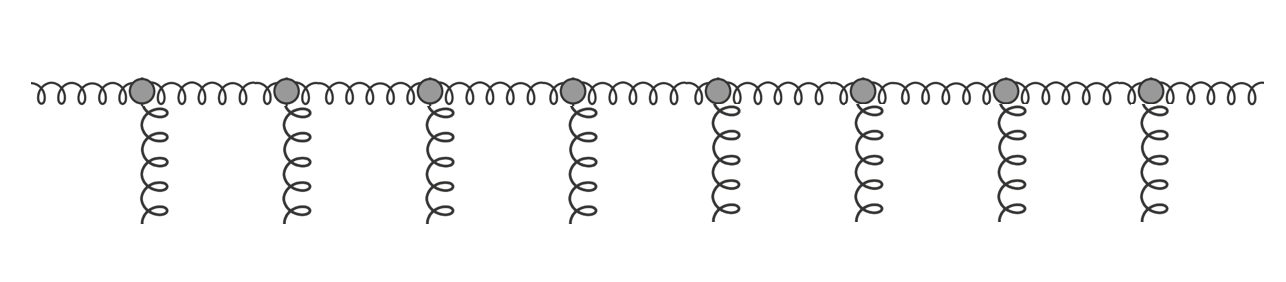
- The horizontal springs again assure continuity — they prevent neighboring balls from moving too far apart, and keep the set of balls behaving like a string.
- The vertical springs provide a restoring effect — they pull or push each ball back toward the position it holds in the figure.
It’s the restoring effect that gives this system unfamiliar standing waves.
Compare The WavesThese systems can exhibit many types of waves, depending on whether their ends are fixed or allowed to float (“boundary conditions”). We can have some fun with all the different options at another time. But today I just want to convince you of the most important thing: that the first system of balls and springs requires walls for its standing waves, while the second one does not.
I’ll make waves analogous to the ones I made in last week’s post on this subject. In the animations below, horizontal springs are drawn as orange lines, while vertical ones are drawn as black lines.
First, let’s take the system with only horizontal springs, distort it upward only in the middle, and let go. No simple standing wave results; we get two traveling waves moving in opposite directions and reflecting off the walls (shown as red, fixed dots.)
Now let’s take the system that has vertical springs as well. In particular, let’s make the vertical springs strong, so that the restoring effect is powerful. Again, let’s distort the system upward at the center, and let go. Now the restoring force of the vertical springs creates a standing wave. That wave is nowhere near the walls, and doesn’t care that there are walls at all. It gradually spreads out, but maintains its coherence for many vibration cycles.
The stronger the vertical springs compared to the horizontal springs, the faster the vibration will be, and the slower the spreading of the wave — and thus the longer the standing wave will maintain its integrity.
The Profound Importance of the Restoring EffectThe key difference, then, between the two systems is the existence of the restoring effect of the vertical springs. More specifically, the two types of springs battle it out, the restoring effect fighting the continuity effect. Whether the former wins or the latter wins is what determines whether the system has long-lasting unfamiliar standing waves that require no walls.
In school and in music, we only encounter systems where the restoring effect is absent, and the continuity effect is dominant. But our very lives depend on the existence of a restoring effect for many of nature’s fields. That effect provides the key difference between photons and electrons (see chapters 17 and 20) — the electromagnetic field, whose ripples are photons, experiences no restoring effect, while the electron field, whose ripples are electrons, is subject to a significant restoring effect.
As described in chapter 20 of the book (which gives other examples of a systems with unfamiliar standing waves), this restoring effect is intimately tied to the workings of the Higgs field.
Likelihood of Auroras Tonight (March 24-25)
[Note Added: 9:30pm Eastern] Unfortunately this storm has consisted of a very bright spike of high activity and a very quick turnoff. It might restart, but it might not. Data below shows recorded activity in three-hour intervals — and the red or very high orange is where you’d want things to be for mid-latitude auroras.
The current solar storm has so far only had a high but brief spike, and might be over already.
Quick note: a powerful double solar flare from two groups of sunspots occurred on Friday. This in turn produced a significant blast of subatomic particles and magnetic field, called a Coronal Mass Ejection [CME], which headed in the direction of Earth. This CME arrived at Earth earlier than expected — a few hours ago — which also means it was probably stronger than expected, too. For those currently in darkness and close enough to the poles, it is probably generating strong auroras, also known as the Northern and Southern Lights.
No one knows how long this storm will continue, but check your skies tonight if you are in Europe especially, and possibly North America as well. The higher your latitude and the earlier your nightfall compared to now, the better your chances.
The ACE satellite, located between the Earth and Sun at a distance from Earth approximately 1% of the Sun-Earth distance, recorded the arrival of the CME a few hours ago as a jump in a number of its readings.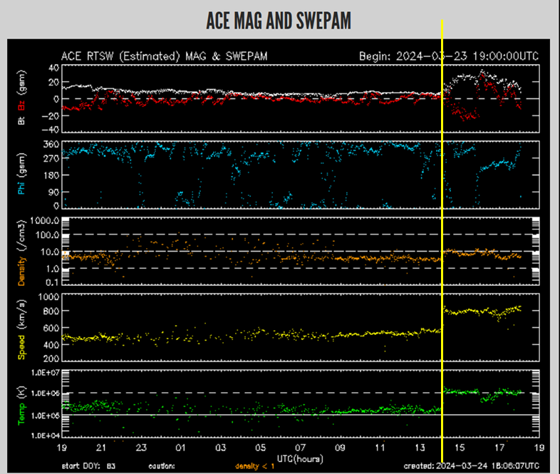
What are Fields?
One of the most challenging aspects of writing a book or blog about the universe (as physicists currently understand it) is that both writer and reader must confront the concept of fields. The problem isn’t that fields are intrinsically that complicated. It’s that they are an unfamiliar abstraction — and novel abstractions of any sort are always difficult both for a writer to describe and for a reader to grasp.
What I’ll do today is give an explanation of fields that is complementary to the one that appears in the book’s chapters 13 and 14. The book’s approach is slow, methodical, and detailed, but today’s will be more of an overview, brief and relatively shallow, and presented in a different order. You will likely come away with many unanswered questions, but the book should help with that. And if the book and today’s post combined are still not enough, you can ask a question in the comments below, or on the book question page.
Negotiating the Abstract and the ConcreteTo approach an abstract concept, it’s always good to have concrete examples. The first example of a field of the cosmos that comes to mind, one that most people have heard of and encountered, is the magnetic field. Unfortunately, it’s not all that concrete. For most of us, it’s near-magic: we can see and feel that it somehow makes little metal blocks cluster together or stick to refrigerator doors, but the field itself remains remote from human experience, as it can’t be seen or felt directly.
There are fields, however, that are less magic-seeming and are known to everyone. The most obvious, though it often goes unrecognized, is the “wind field” of the atmosphere. Since we all experience it, and since weather maps often depict it, that’s the field I focused on in the book’s chapter 13. I hoped that by using it as an initial example, it would make the concept of “field” more intuitive for many readers.
But I knew that inevitably, no matter what approach I chose, it wouldn’t work for all readers. (My own father, for instance, has had more trouble making sense of that part of the book than any other.) Knowing this would happen, I’ve planned from the beginning to give alternate explanations here, to offer readers multiple roads into this unfamiliar concept.
Ordinary FieldsIn general, I find that the fields of the universe — I’ll call them “cosmic fields”, for short — are not the best starting point. That’s because they are mostly unfamiliar, and are intrinsically confusing and obscure even to physicists.
Instead, I’ll start with fields of ordinary materials, like water, air, rock and iron. We will see there is an interesting analogy between the fields of materials and the fields of the cosmos, one which will give us a great deal of useful intuition.
However, this analogy comes with a strongly-worded caution, warning and disclaimer, because the cosmos has properties that no ordinary material could possibly have. (See chapter 14 for a detailed discussion.) For this reason, please be careful not to take the analogy to firmly to heart. It has many merits, but we will definitely have to let some of it go — and perhaps all of it.
Air and its FieldsSo let’s start with a familiar material and its properties: the air that makes up the Earth’s atmosphere, and some of the properties of the air that are recorded by weather stations. As I write this, the weather station at Boston’s Logan Airport is reporting on conditions there, stating that it measures
- Wind W 10 mph
- Pressure 29.71 in (1005.8 mb)
- Humidity 43%
There are similar weather stations scattered about the world that give us information about wind, pressure and humidity at various locations. But we don’t have complete information; obviously we don’t have weather stations at every point in the atmosphere!
Nevertheless, at all times, every point in the atmosphere does in fact have its own wind, pressure, and humidity, even if there’s no weather station there to measure it. Each of these properties of the air is meaningful throughout the atmosphere, varies from place to place, and changes over time.
Now we make our first step into abstraction. We can define the air’s property of pressure, viewed all across the atmosphere, as a field. When we do this, we view the pressure not as something measured at a particular place and time but as if it were measured everywhere in space and time. This makes it into a function of space and time — a function that tells us the pressure at all points in the atmosphere and at all times in Earth’s history. If we define x,y,z to be three coordinates that specify where we are in the three-dimensional atmosphere, and t to be a coordinate that specifies what time it is, then the pressure at that particular place and time can be written as P(x,y,z,t) — a function that takes in a position and a time and outputs the pressure at that position and time.
For instance, consider the point (xB,yB,zB) corresponding to Logan airport, and the time t0 when I was writing this article. According to the weather station whose measurements I reported above, the value of the pressure field at that position and moment, P(xB, yB, zB, t0), was equal to 29.71 inches of mercury (or, equivalently, 1005.8 millibarns).
Any one weather station’s report tells us only what the pressure is at a particular location and moment. But if we knew the pressure field perfectly at a moment t — if we had complete knowledge of the function P(x,y,z,t) — we’d know how strong the pressure is everywhere in the atmosphere at that moment.
In a similar way, we can define the “wind field” and the “humidity field” (or “water-vapor density field”) to capture what the wind and humidity are doing across the atmosphere’s entire expanse. Each field’s value at a particular location and time tells us what a measurement of the corresponding property would show at that location and time.
Maps and images illustrating three atmospheric fields: (top to bottom) air pressure, average wind patterns, and water vapor (humidity). Credits: NOAA.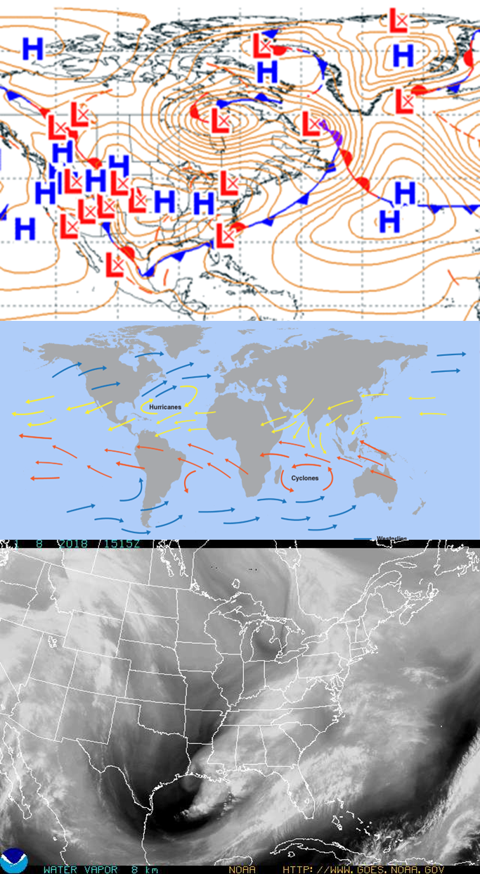
These three fields interact with each other, with other fields, and with external effects (such as sunlight) to create weather. Detailed weather forecasting is only possible because scientists have largely understood how these fields behave and how they affect one another, and have expressed their understanding through math equations that have been programmed into weather forecasting computers.
Air as a MediumAbstracting even further, we may think of the air of the atmosphere as an example of what one would call an ordinary medium — a largely uniform substance that occupies a wide area for an extended period of time. The water of the oceans is another example of an ordinary medium. Others include the rock of the Earth, the plasma that makes up the Sun, the gas of Jupiter’s atmosphere, a large block of iron or copper or lead, the pure neutron material of a neutron star, and so on.
Each medium has a number of properties, just as air does. Its properties that vary from place to place and change predictably with time can be viewed as fields, in the same way that air pressure and wind can be viewed as fields.
And so we reach a highly abstract level: an ordinary field is
- a property of an ordinary medium . . .
- that can be measured, . . .
- varies from place to place, . . .
- and changes with time in a manner that (at least in principle) is predictable.
Let’s look at a few examples to make this more concrete.
- For the oceans, fields include the current (the flow of the water) and the water pressure.
- The fields of layered sedimentary rock include the rock’s density and the degree to which (and direction in which) its layers have been bent.
- For a block of iron, fields include the iron’s density (the number of atoms in a cube of material divided by the cube’s volume), the orientation of its crystal structure (which might be bent in places), and the average local orientation of its atoms; the latter, usually called the “magnetization field”, determines if the iron will act as a magnet or not.
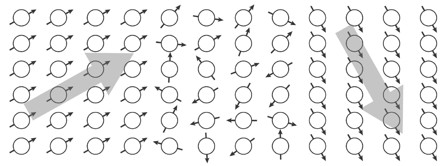
This manner of thinking is a commonplace, and a powerful one, for physicists who spend their careers studying ordinary materials, such as metals, superconductors, fluids, and so on. Each type of ordinary medium has ordinary fields that characterize it, and these fields interact with each other in ways that are specific to that medium. In some cases, even if we knew nothing about the medium, knowing all its fields and all their interactions with one another might allow us to guess what the medium is.
Cosmic FieldsWe can now turn to the cosmos itself. Over the last two centuries, physicists have found that there are quite a few quantities that can be measured everywhere and at all times, that vary from place to place and from moment to moment, and that affect one another. These quantities have also been called “fields”. Just to be clear, I’ll call them “cosmic fields” to distinguish them from the “ordinary fields” that we have just been discussing.
In many ways, cosmic fields resemble ordinary fields. They act in many ways as though the cosmos were a medium, and as though the fields represent some of the properties of that medium.
Empty Space as a MediumEinstein himself gave us a good reason to think along these lines. In his approach to gravity, known as general relativity, the empty space that pervades the universe should be viewed as a sort of medium. (That includes the space inside of objects, such as our own bodies.) Much as pressure represents a property of air, Einstein’s gravitational field (which generates all gravitational effects) represents a property of space — the degree to which space is bent. We often call that property the “curvature” or “warping” of space.
The list of cosmic fields is extensive, and includes the electromagnetic field and the Higgs field among others. Should we think of each of these fields as representing an additional property of empty space?
Maybe that’s the right way to think about these other cosmic fields. But we must be wary. We don’t yet have any evidence that this is the right viewpoint.
The Fields of Empty Space?This brings us to the greatest abstraction of all, the one that physicists live with every day.
- Cosmic fields may be properties of the medium that we call “empty space”. Or they may not be.
- Even if they are, though, we have no idea (with the one exception of the gravitational field) what properties they correspond to. Our understanding of empty space is still far too limited.
This tremendous gap in our understanding might seem to leave us completely at sea. But fortunately, physicists have learned how to use measurement and math to make predictions about how the cosmic fields behave despite having no understanding what properties of empty space these fields might represent. Even though we don’t know what the cosmic fields are, we have extensive knowledge and understanding of what they do.
An Analogy Both Useful And ProblematicIt may seem comforting, if a bit counterintuitive, to imagine that the universe’s empty space might in fact be a something — a sort of substance, much as air and rock are substances — and that this cosmic substance, like air and rock, has properties that can be viewed as fields. From this perspective, a central goal of modern theoretical physicists who study particles and fields is the following: to figure out what the cosmos is made from and what properties the various fields correspond to.
Imagine that it was your job to start from weather reports that look like this:
- Field A: W 18 mph
- Field B: 29.62 in (1003.0 mb)
- Field C: 63%
and then try to deduce, from a huge number of these reports, what the atmosphere is made from and what properties the fields called “A”, “B” and “C” correspond to. This is akin to what today’s physicists have to do. We have discovered various fields that we can measure and study, and to which we’ve given arbitrary names; and we’d like to infer from their behavior what empty space really is and what its fields actually represent.
This is an interesting way to think about what particle physicists are doing nowadays. But we should be careful not to take it too seriously.
- First, the whole analogy, tempting as it is, might be completely wrong. It may be that the fields of the universe represent something completely different from the ordinary properties of an ordinary medium, and that the seeming similarity of the two is deeply misleading.
- Second, the analogy is definitely wrong in part: we already know that the universe cannot be like an ordinary medium. That’s a long story (explained carefully in the book’s chapter 14), but the bottom line is that empty space has properties that no ordinary medium can possibly have.
Nevertheless, the notion that ordinary media made from ordinary materials have ordinary fields, and that empty space has cosmic fields that bear some rough resemblance to what we see in ordinary media, is useful. The analogy helps us gain some basic intuition for how fields work and for what they might be, even though we have to remain cautious about its flaws, known and unknown. This manner of thinking was useful to Einstein in the research of his later years (even though it led to a dead end), and it also arises naturally in string theory (which may or may not be a dead end.)
Whether, in the long run, this analogy proves more beneficial than misleading is something that only future research will reveal. But for now, I think it can serve experts and non-experts alike, as long as we keep in mind that it cannot be the full story.
Yes, Standing Waves Can Exist Without Walls
After my post last week about familiar and unfamiliar standing waves — the former famous from musical instruments, the latter almost unknown except to physicists (see Chapter 17 of the book) — I got a number of questions. Quite a few took the form, “Surely you’re joking, Mr. Strassler! Obviously, if you have a standing wave in a box, and you remove the box, it will quickly disintegrate into traveling waves that move in opposite directions! There is no standing wave without a container.”
Well, I’m not joking. These waves are unfamiliar, sure, to the point that they violate what some readers may have learned elsewhere about standing waves. Today I’ll show you animations to prove it.
When a Standing Wave Loses Its BoxThe animations below show familiar and unfamiliar standing waves inside small boxes (indicated in orange). The boxes are then removed, leaving the waves to expand into larger boxes. What happens next is determined by straightforward math; if you’re interested in the math, see the end of this post.
Though the waves start out with the same shape, they have different vibrational frequencies; the unfamiliar wave vibrates ten times faster. Each wave vibrates in place until the small box is taken away. Then the familiar wave instantly turns into two traveling waves that move in opposite directions at considerable speed, quickly reaching and reflecting off the walls of the new box. Nothing of the original standing wave survives, except that its ghost is recreated for a moment when the two traveling waves intersect.
The unfamiliar wave, however, has other plans. It continues to vibrates at the center of the box for quite a while, maintaining its coherence and only slowly spreading out. As the traveling waves from the familiar standing wave are hitting the walls of the outer box, the unfamiliar wave is still just barely tickling those walls. Only at the very end of the animation is this wave even responding of the presence of the box.
A familiar standing wave vibrates within a small box. When the small box is removed, the wave decomposes into traveling waves that reflect off the walls of the larger box. Animation made using Mathematica. Same as at left, but for an unfamiliar standing wave. For the same shape, it initially has a higher frequency, and it spreads much more slowly when the smaller box is removed. Animation made using Mathematica.
To fully appreciate this effect, imagine if I’d made the ratio between the two waves’ frequencies one thousand instead of ten. Then the unfamiliar wave would have taken a thousand times longer than the familiar wave to completely spread across its box. However, I didn’t think you’d want to watch such boring animations, so I chose a relatively small frequency ratio.
Now let’s put in some actual numbers, to appreciate how impressive this becomes when applied to real particles.
Photons and Electrons in BoxesLet’s take an empty box (having removed the air inside it) whose sides are a tenth of a meter (about three inches) long. If I put a standing-wave photon (a particle of light) into it, that wave will have a frequency of 3 billion cycles per second. That puts it in the microwave range.
If I then release the photon into a box a full meter across, the photon’s wave will turn into traveling pulses, as my first animation showed. Moving at the speed of light, the pulses will reach the walls of the larger box in about 1.5 billionths of a second (1.5 nanoseconds.) This is what we are taught to expect: without the walls, the standing wave can’t survive.
But if I put a standing-wave electron in a box a tenth of a meter across, it will have a frequency of 800 billion billion cycles per second. That’s not a typo — I really do mean 800 Billion-Billion, which is enormously faster vibration than for a microwave photon.
Correspondingly, when the electron is released from its original box to a larger one a meter across, it will simply remain vibrating at the center of the box, in an extreme version of the second animation. The edges of the electron’s wave will expand, but no faster than a few millimeters per second. The amount of time it will take for its vibrating edges to reach out to the edges of the new box will be well over a minute.
From the electron’s perspective, vibrating once every billionth of a trillionth of a second, this spreading takes almost forever. It’s a long time even for a human physicist. Most experiments on freely floating electrons, including those that measure an electron’s rest mass, take much less than a second. For many such measurements, the fact that an unconstrained electron is gradually spreading is of little practical importance.
Atoms are Boxes TooThus standing waves can exist without walls for a quite a while, if they are sufficiently broad to start with. The word broad is important here. From smaller boxes, or from atoms, the spreading is more rapid; an electron liberated from a tiny hydrogen atom can grow to the size of a room in the blink of an eye. The larger the electron’s initial container, the wider the electron’s initial standing wave will be, and the more slowly it will spread.
This pattern might remind you of the famous and infamous uncertainty principle. And well it should.
For the math behind this, read this article (the fourth of this series); the familiar waves satisfy what I called Class 0 wave equations, while the unfamiliar ones satisfy Class 1 wave equations. If you read to the end of the series, you’ll see the direct connection of these two classes of waves with photons and electrons, and more generally with particles of zero and non-zero rest mass.